This notebook builds the geometric and algebraic understanding of the determinant from first principles, culminating in why $\det(A) = 0$ is the exact condition for singularity.
import numpy as np
import matplotlib.pyplot as plt
import matplotlib.patches as mpatches
from matplotlib.patches import Polygon
from matplotlib.collections import PatchCollection

def style_ax(ax, title='', xlim=(-4, 4), ylim=(-4, 4)):
    ax.set_xlim(*xlim); ax.set_ylim(*ylim)
    ax.set_aspect('equal')
    ax.axhline(0, color='gray', lw=0.7)
    ax.axvline(0, color='gray', lw=0.7)
    ax.set_title(title, fontsize=11, pad=8)
    ax.set_xlabel('$x_1$'); ax.set_ylabel('$x_2$')
    ax.grid(True, linestyle='--', alpha=0.3)

def draw_arrow(ax, vec, origin=None, color='black', lw=2, label=None, offset=None):
    o = np.zeros(2) if origin is None else np.array(origin)
    ax.annotate('', xy=o + vec, xytext=o,
                arrowprops=dict(arrowstyle='->', color=color, lw=lw))
    if label:
        pos = o + vec + (offset if offset is not None else np.array([0.1, 0.1]))
        ax.text(*pos, label, color=color, fontsize=12, fontweight='bold')

def draw_parallelogram(ax, c1, c2, color='steelblue', alpha=0.25, edge_lw=1.5):
    """Draw the parallelogram spanned by two column vectors."""
    corners = np.array([[0,0], c1, c1+c2, c2, [0,0]])
    ax.fill(corners[:,0], corners[:,1], color=color, alpha=alpha)
    ax.plot(corners[:,0], corners[:,1], color=color, lw=edge_lw)
1. The Determinant as a Volume Scaling Factor
The most fundamental interpretation of the determinant is geometric, not algebraic:
$\det(A)$ is the signed volume of the parallelepiped formed by the columns of $A$.
In 2D, this is the signed area of the parallelogram spanned by the two column vectors $a_1$ and $a_2$:
$$A = \begin{bmatrix} | & | \ a_1 & a_2 \ | & | \end{bmatrix}, \qquad \det(A) = \text{signed area of parallelogram}(a_1, a_2)$$
More broadly, when $A$ is applied to any region $S$ of space:
$$\text{Vol}(A \cdot S) = |\det(A)| \cdot \text{Vol}(S)$$
The determinant is a uniform volume scaling factor — it tells you by how much the transformation stretches or compresses all of space.
# Three matrices: stretch, compress, identity
matrices = [
    (np.eye(2),                        'Identity\n$\\det = 1$'),
    (np.array([[2., 1.],[0.5, 1.5]]),   'Non-singular\n$\\det = {:.2f}$'.format(np.linalg.det(np.array([[2.,1.],[0.5,1.5]])))),
    (np.array([[0.5, 0.],[0.,  0.5]]), 'Uniform compression\n$\\det = {:.2f}$'.format(np.linalg.det(np.array([[0.5,0.],[0.,0.5]])))),
]

# Unit square
unit_sq = np.array([[0,1,1,0,0],[0,0,1,1,0]], dtype=float)

fig, axes = plt.subplots(1, 3, figsize=(15, 5))
for ax, (M, title) in zip(axes, matrices):
    c1, c2 = M[:, 0], M[:, 1]
    draw_parallelogram(ax, c1, c2, color='steelblue')
    draw_arrow(ax, c1, color='crimson',    lw=2.5, label='$a_1$', offset=np.array([ 0.1, -0.3]))
    draw_arrow(ax, c2, color='darkorange', lw=2.5, label='$a_2$', offset=np.array([ 0.1,  0.1]))
    area = abs(np.linalg.det(M))
    ax.text(0.05, 0.95, f'Area = {area:.2f}', transform=ax.transAxes,
            fontsize=10, va='top', bbox=dict(boxstyle='round', facecolor='wheat', alpha=0.5))
    style_ax(ax, title=title, xlim=(-0.5, 3.5), ylim=(-0.5, 2.5))

fig.suptitle('The determinant = signed area of the parallelogram spanned by the columns', fontsize=13)
plt.tight_layout()
plt.show()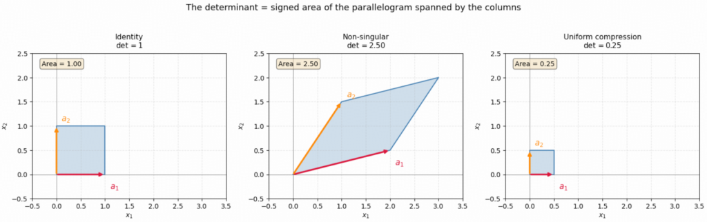
2. The Sign Encodes Orientation
The determinant is signed. The sign indicates whether the transformation preserves or reverses orientation:
| $\det(A)$ | Volume effect | Orientation |
|---|---|---|
| $> 0$ | Scales by $\det(A)$ | Preserved |
| $< 0$ | Scales by $ | \det(A) |
| $= 0$ | Destroyed | Undefined |
A negative determinant means the transformation includes a reflection — the columns have swapped their relative handedness compared to the standard basis.
A_pos = np.array([[ 2.0,  0.5], [0.5, 1.5]])   # det > 0
A_neg = np.array([[-2.0,  0.5], [0.5, 1.5]])   # det < 0  (col 1 reflected)

fig, axes = plt.subplots(1, 3, figsize=(15, 5))

# Standard basis reference
ax = axes[0]
draw_parallelogram(ax, np.array([1.,0.]), np.array([0.,1.]), color='gray')
draw_arrow(ax, np.array([1.,0.]), color='crimson',    lw=2.5, label='$e_1$', offset=np.array([0.05,-0.25]))
draw_arrow(ax, np.array([0.,1.]), color='darkorange', lw=2.5, label='$e_2$', offset=np.array([-0.3, 0.1]))
ax.text(0.3, 0.3, 'CCW', fontsize=11, color='gray')
style_ax(ax, title='Standard basis\n$\\det(I) = +1$ (reference)', xlim=(-2.5,2.5), ylim=(-2.5,2.5))

# Positive determinant
ax = axes[1]
c1, c2 = A_pos[:,0], A_pos[:,1]
draw_parallelogram(ax, c1, c2, color='steelblue')
draw_arrow(ax, c1, color='crimson',    lw=2.5, label='$a_1$', offset=np.array([ 0.1,-0.3]))
draw_arrow(ax, c2, color='darkorange', lw=2.5, label='$a_2$', offset=np.array([ 0.1, 0.1]))
d = np.linalg.det(A_pos)
ax.text(0.5, 0.5, 'CCW', fontsize=11, color='steelblue')
style_ax(ax, title=f'$\\det(A) = +{d:.2f}$\nOrientation preserved', xlim=(-2.5,3.5), ylim=(-0.5,3.5))

# Negative determinant
ax = axes[2]
c1, c2 = A_neg[:,0], A_neg[:,1]
draw_parallelogram(ax, c1, c2, color='mediumorchid')
draw_arrow(ax, c1, color='crimson',    lw=2.5, label='$a_1$', offset=np.array([-0.6,-0.3]))
draw_arrow(ax, c2, color='darkorange', lw=2.5, label='$a_2$', offset=np.array([ 0.1, 0.1]))
d = np.linalg.det(A_neg)
ax.text(-1.0, 0.5, 'CW', fontsize=11, color='mediumorchid')
style_ax(ax, title=f'$\\det(A) = {d:.2f}$\nOrientation reversed (reflection)', xlim=(-3.5,2.5), ylim=(-0.5,3.5))

fig.suptitle('Sign of the determinant encodes orientation', fontsize=13)
plt.tight_layout()
plt.show()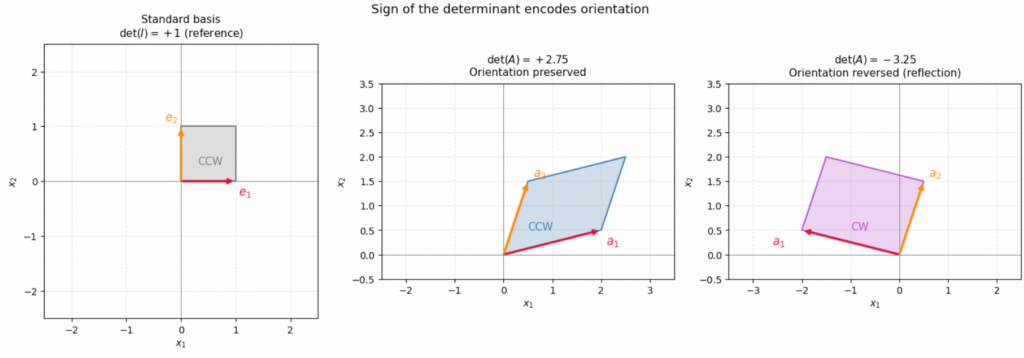
3. Why $\det(A) = 0$ Means Singular: Dimension Collapse
When $\det(A) = 0$, the transformation maps $\mathbb{R}^n$ into a strictly lower-dimensional subspace. In 2D, the entire plane gets flattened onto a line (or a point). The parallelogram has zero area because the two column vectors are collinear — they both point along the same line.
$$\det(A) = 0 \iff \text{columns of } A \text{ are linearly dependent} \iff \text{image of } A \text{ has dimension} < n$$
# Singular matrix: col2 = 2 * col1
A_sing = np.array([[1.0, 2.0],
                   [0.5, 1.0]])

# A grid of input points
grid_pts = np.array([[x, y] for x in np.linspace(-2,2,9)
                             for y in np.linspace(-2,2,9)]).T
transformed = A_sing @ grid_pts

fig, axes = plt.subplots(1, 2, figsize=(13, 5))

# Input space
ax = axes[0]
ax.scatter(grid_pts[0], grid_pts[1], color='steelblue', s=30, zorder=3)
draw_arrow(ax, A_sing[:,0], color='crimson',    lw=2.5, label='$a_1$', offset=np.array([ 0.1,-0.25]))
draw_arrow(ax, A_sing[:,1], color='darkorange', lw=2.5, label='$a_2 = 2a_1$', offset=np.array([0.1, 0.1]))
style_ax(ax, title='Input: 2D grid of points', xlim=(-3,3), ylim=(-3,3))

# Output space — everything collapses to a line
ax = axes[1]
ax.scatter(transformed[0], transformed[1], color='crimson', s=30, zorder=3, label='Transformed points')
# draw the line that the space collapsed onto
t = np.linspace(-4, 4, 100)
col1 = A_sing[:, 0]
ax.plot(col1[0]*t, col1[1]*t, 'k--', lw=1.5, alpha=0.5, label='Image: 1D line (col space)')
ax.legend(fontsize=9)
style_ax(ax, title=f'Output: entire 2D plane collapses to a 1D line\n$\\det(A) = {np.linalg.det(A_sing):.4f} \\approx 0$',
         xlim=(-4,4), ylim=(-3,3))

fig.suptitle('Singular matrix: $a_2 = 2a_1$ — columns are linearly dependent', fontsize=13)
plt.tight_layout()
plt.show()

print(f"A_sing =\n{A_sing}")
print(f"det(A_sing) = {np.linalg.det(A_sing):.6f}")
print(f"rank(A_sing) = {np.linalg.matrix_rank(A_sing)}  (collapsed from 2 to 1)")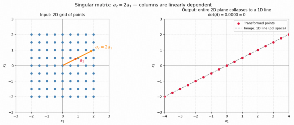
A_sing =
[[1.  2. ]
 [0.5 1. ]]
det(A_sing) = 0.000000
rank(A_sing) = 1  (collapsed from 2 to 1)
4. The Mechanism: Alternating Multilinearity
Why does linear dependence force $\det = 0$? The answer lies in two algebraic properties that define the determinant:
Multilinear — scaling any one column scales the determinant by the same factor:
$$\det([\ldots, \alpha a_j, \ldots]) = \alpha \cdot \det([\ldots, a_j, \ldots])$$
Alternating — swapping any two columns negates the determinant, and a repeated column gives zero:
$$\det([\ldots, a_i, \ldots, a_i, \ldots]) = 0$$
Now suppose column $k$ is a linear combination of the others: $a_k = \sum_{j \neq k} c_j a_j$. By multilinearity, the determinant expands into a sum of terms — each one containing a repeated column. The alternating property kills each term. Therefore:
$$a_k \in \text{span}(\text{other columns}) \implies \det(A) = 0$$
# Demonstrate: gradually make col2 more dependent on col1 and watch det → 0
a1 = np.array([1.0, 0.5])
a2_original = np.array([0.5, 2.0])   # independent
a2_dependent = 2.0 * a1              # col2 = 2*col1

alphas = np.linspace(0, 1, 200)
dets = []
for alpha in alphas:
    a2 = (1 - alpha) * a2_original + alpha * a2_dependent
    M = np.column_stack([a1, a2])
    dets.append(np.linalg.det(M))

fig, axes = plt.subplots(1, 2, figsize=(13, 4))

# Left: det vs interpolation
ax = axes[0]
ax.plot(alphas, dets, color='steelblue', lw=2)
ax.axhline(0, color='crimson', lw=1.5, linestyle='--', label='$\\det = 0$ (singular)')
ax.scatter([0, 1], [dets[0], dets[-1]], s=80, zorder=5,
           color=['green', 'crimson'], label=['Independent', 'Fully dependent'])
ax.set_xlabel('$\\alpha$ (0 = independent, 1 = fully dependent)')
ax.set_ylabel('$\\det(A)$')
ax.set_title('Determinant as $a_2 \\to 2a_1$')
ax.legend(fontsize=9)
ax.grid(True, alpha=0.3)

# Right: parallelogram shrinking
ax = axes[1]
for alpha in [0, 0.33, 0.66, 1.0]:
    a2 = (1 - alpha) * a2_original + alpha * a2_dependent
    corners = np.array([[0,0], a1, a1+a2, a2, [0,0]])
    color = plt.cm.RdYlGn(1 - alpha)
    ax.fill(corners[:,0], corners[:,1], color=color, alpha=0.35)
    ax.plot(corners[:,0], corners[:,1], color=color, lw=1.5,
            label=f'$\\alpha={alpha:.2f}$, area={abs((1-alpha)*dets[0]):.2f}')
draw_arrow(ax, a1, color='black', lw=2, label='$a_1$ (fixed)', offset=np.array([0.05,-0.2]))
ax.legend(fontsize=8, loc='upper left')
style_ax(ax, title='Parallelogram area collapsing to zero', xlim=(-0.3, 3.5), ylim=(-0.3, 2.5))

plt.tight_layout()
plt.show()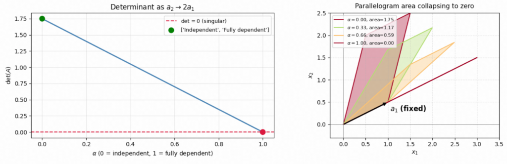
5. The Invertibility Connection
A matrix $A$ is invertible iff $Ax = b$ has a unique solution for every $b$. This fails when $A$ collapses a dimension — either outputs are unreachable, or multiple inputs share the same output.
The product rule $\det(AB) = \det(A)\det(B)$ makes the impossibility of inverting a singular matrix algebraically transparent:
$$I = AA^{-1} \implies 1 = \det(I) = \det(A)\det(A^{-1})$$
If $\det(A) = 0$, this demands $0 \cdot \det(A^{-1}) = 1$ — a contradiction. No $A^{-1}$ can exist.
# Visualise the null space: Ax = 0 has non-trivial solutions when det = 0
fig, axes = plt.subplots(1, 2, figsize=(13, 5))

A_inv  = np.array([[2.0, 0.5], [0.5, 1.5]])   # invertible
A_sing = np.array([[1.0, 2.0], [0.5, 1.0]])   # singular

grid_x = np.linspace(-3, 3, 300)

for ax, (M, title) in zip(axes, [
    (A_inv,  f'Non-singular ($\\det={np.linalg.det(A_inv):.2f}$)\nNull space = {{0}} only'),
    (A_sing, f'Singular ($\\det={np.linalg.det(A_sing):.4f}$)\nNull space is a full line'),
]):
    # Show column space
    c1, c2 = M[:,0], M[:,1]
    draw_parallelogram(ax, c1, c2, color='steelblue', alpha=0.15)
    draw_arrow(ax, c1, color='crimson',    lw=2.5, label='$a_1$', offset=np.array([ 0.1,-0.3]))
    draw_arrow(ax, c2, color='darkorange', lw=2.5, label='$a_2$', offset=np.array([ 0.1, 0.1]))

    # Null space: solve Mx = 0
    _, _, Vt = np.linalg.svd(M)
    null_dim = M.shape[1] - np.linalg.matrix_rank(M)
    if null_dim > 0:
        null_vec = Vt[-1]   # last row of Vt = null space basis vector
        t = np.linspace(-3, 3, 100)
        ax.plot(null_vec[0]*t, null_vec[1]*t, 'purple', lw=2.5,
                label=f'Null space: all $x$ with $Ax=0$')
        # verify
        print(f"Null space vector: {null_vec.round(4)}")
        print(f"A @ null_vec = {(M @ null_vec).round(6)}  (≈ 0 ✓)\n")
    else:
        ax.scatter([0],[0], color='purple', s=100, zorder=5, label='Null space: {0} only')
        print(f"Non-singular: only Ax=0 solution is x=0 ✓\n")

    ax.legend(fontsize=9)
    style_ax(ax, title=title, xlim=(-3,3), ylim=(-3,3))

fig.suptitle('Null space of $A$: trivial (invertible) vs. a full line (singular)', fontsize=13)
plt.tight_layout()
plt.show()
Non-singular: only Ax=0 solution is x=0 ✓
Null space vector: [ 0.8944 -0.4472]
A @ null_vec = [0. 0.] (≈ 0 ✓)
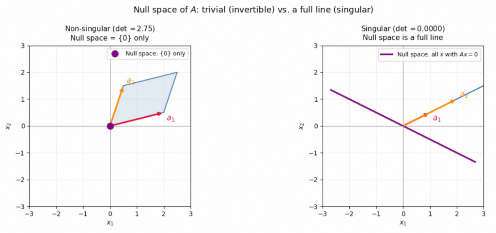
6. Determinant and Eigenvalues
The determinant equals the product of all eigenvalues:
$$\det(A) = \prod_{i=1}^{n} \lambda_i$$
This gives another route to the same conclusion: $\det(A) = 0$ iff at least one $\lambda_i = 0$. A zero eigenvalue means some nonzero vector $v$ satisfies $Av = 0 \cdot v = 0$ — it gets annihilated by the transformation. That is exactly a nontrivial null space.
And since singular values $\sigma_i = \sqrt{\lambda_i(A^\top A)}$, a zero singular value is the same condition expressed through the SVD lens.
for M, name in [(A_inv, 'Non-singular'), (A_sing, 'Singular')]:
    eigvals = np.linalg.eigvals(M)
    singular_vals = np.linalg.svd(M, compute_uv=False)
    det_direct   = np.linalg.det(M)
    det_via_eigs = np.prod(eigvals).real

    print(f"=== {name} ===")
    print(f"  Eigenvalues    : {np.round(eigvals.real, 4)}")
    print(f"  det (direct)   : {det_direct:.6f}")
    print(f"  det (∏ λᵢ)     : {det_via_eigs:.6f}  ✓")
    print(f"  Singular values: {np.round(singular_vals, 6)}")
    print(f"  Rank           : {np.linalg.matrix_rank(M)}")
    print()
=== Non-singular === Eigenvalues : [2.309 1.191] det (direct) : 2.750000 det (∏ λᵢ) : 2.750000 ✓ Singular values: [2.309017 1.190983] Rank : 2 === Singular === Eigenvalues : [2. 0.] det (direct) : 0.000000 det (∏ λᵢ) : 0.000000 ✓ Singular values: [2.5 0. ] Rank : 1
7. All Equivalent Conditions — Unified View
Every condition below describes the same underlying geometric fact: the transformation collapses at least one dimension.
def audit(M, name):
    eigvals = np.linalg.eigvals(M)
    svals   = np.linalg.svd(M, compute_uv=False)
    rank    = np.linalg.matrix_rank(M)
    n       = M.shape[0]
    det     = np.linalg.det(M)
    null_trivial = rank == n   # Ax=0 has only x=0

    print(f"{'='*55}")
    print(f" {name}")
    print(f"{'='*55}")
    print(f"  det(A)                      : {det:.6f}")
    print(f"  Rank = n ({n})?              : {rank == n}  (rank = {rank})")
    print(f"  All eigenvalues ≠ 0?        : {all(abs(eigvals) > 1e-10)}  {np.round(eigvals.real, 4)}")
    print(f"  All singular values > 0?    : {all(svals > 1e-10)}  {np.round(svals, 6)}")
    print(f"  Null space trivial ({{0}})?   : {null_trivial}")
    try:
        np.linalg.inv(M)
        invertible = True
    except np.linalg.LinAlgError:
        invertible = False
    print(f"  Invertible?                 : {invertible}")
    print()

audit(A_inv,  'Non-singular A')
audit(A_sing, 'Singular A')
=======================================================
Non-singular A
=======================================================
det(A) : 2.750000
Rank = n (2)? : True (rank = 2)
All eigenvalues ≠ 0? : True [2.309 1.191]
All singular values > 0? : True [2.309017 1.190983]
Null space trivial ({0})? : True
Invertible? : True
=======================================================
Singular A
=======================================================
det(A) : 0.000000
Rank = n (2)? : False (rank = 1)
All eigenvalues ≠ 0? : False [2. 0.]
All singular values > 0? : False [2.5 0. ]
Null space trivial ({0})? : False
Invertible? : False
Summary
| Condition | What it says |
|---|---|
| $\det(A) = 0$ | Transformation destroys volume — space is collapsed |
| Columns linearly dependent | At least one column lies in the span of the others |
| $\text{rank}(A) < n$ | Image has lower dimension than domain |
| $Ax = 0$ has nontrivial solutions | Some nonzero vector is annihilated |
| $A$ is not invertible | The transformation cannot be undone |
| At least one eigenvalue $= 0$ | Some direction gets completely flattened |
| At least one singular value $= 0$ | Same condition via SVD |
These are not separate facts. They are one geometric fact — the transformation collapses at least one dimension — expressed from different mathematical viewpoints.
The determinant is the single scalar that captures whether this collapse has occurred: nonzero means the full-dimensional structure of space is preserved and the transformation is reversible; zero means information has been irretrievably lost.
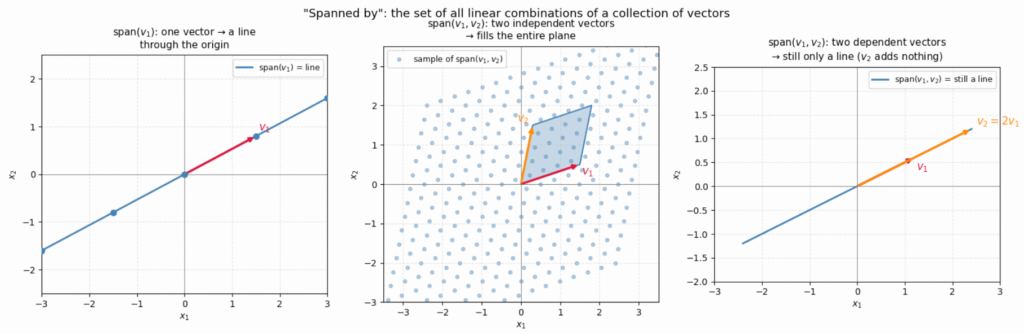
8. What Does “Spanned By” Mean?
The phrase “spanned by” appeared throughout this notebook (e.g. “the parallelogram spanned by $a_1$ and $a_2$”). Here is what it means precisely.
Definition
The span of vectors $v_1, v_2, \ldots, v_k$ is the set of every vector reachable by scaling and adding them in any combination:
$$\text{span}(v_1, v_2, \ldots, v_k) = \left{ \alpha_1 v_1 + \alpha_2 v_2 + \cdots + \alpha_k v_k \;\middle|\; \alpha_i \in \mathbb{R} \right}$$
“The space spanned by $v_1$ and $v_2$” means this entire set — all possible linear combinations.
What spans look like geometrically
| Vectors | Span |
|---|---|
| One nonzero vector in $\mathbb{R}^2$ | A line through the origin |
| Two independent vectors in $\mathbb{R}^2$ | The entire plane $\mathbb{R}^2$ |
| Two dependent vectors in $\mathbb{R}^2$ | Only a line (same as one vector) |
| Three independent vectors in $\mathbb{R}^3$ | All of $\mathbb{R}^3$ |
Key insight: linear dependence shrinks the span. If one vector is already a combination of the others, adding it contributes nothing new.
Connection to this notebook
- “Parallelogram spanned by $a_1$ and $a_2$” — the filled shape formed by all $\alpha_1 a_1 + \alpha_2 a_2$ with $0 \leq \alpha_1, \alpha_2 \leq 1$
- “Column space” — another name for the span of the columns of $A$: all vectors $Ax$ can possibly reach
- “$a_k \in \text{span}(\text{other columns})$” — column $k$ is redundant; it adds no new direction, so the determinant is zero
fig, axes = plt.subplots(1, 3, figsize=(16, 5))

# ── Case 1: span of one vector = a line ─────────────────────────────────────
ax = axes[0]
v1 = np.array([1.5, 0.8])
t = np.linspace(-2.5, 2.5, 200)
span_pts = np.outer(t, v1)                 # all α·v1
ax.plot(span_pts[:, 0], span_pts[:, 1], color='steelblue', lw=2, label='span($v_1$) = line')
# sample a few representative points
for alpha in [-2, -1, 0, 1, 2]:
    pt = alpha * v1
    ax.scatter(*pt, color='steelblue', s=40, zorder=4)
draw_arrow(ax, v1, color='crimson', lw=2.5, label='$v_1$', offset=np.array([0.05, 0.12]))
ax.legend(fontsize=9)
style_ax(ax, title='span($v_1$): one vector → a line\nthrough the origin', xlim=(-3,3), ylim=(-2.5,2.5))

# ── Case 2: span of two independent vectors = the plane ─────────────────────
ax = axes[1]
v1 = np.array([1.5, 0.5])
v2 = np.array([0.3, 1.5])
# shade the reachable region (the whole plane — approximate with a dense grid)
alphas = np.linspace(-2, 2, 18)
pts = np.array([a1*v1 + a2*v2 for a1 in alphas for a2 in alphas])
ax.scatter(pts[:, 0], pts[:, 1], color='steelblue', s=15, alpha=0.4, label='sample of span($v_1, v_2$)')
draw_arrow(ax, v1, color='crimson',    lw=2.5, label='$v_1$', offset=np.array([ 0.05,-0.25]))
draw_arrow(ax, v2, color='darkorange', lw=2.5, label='$v_2$', offset=np.array([-0.4,  0.1]))
# highlight the parallelogram (α ∈ [0,1])
draw_parallelogram(ax, v1, v2, color='steelblue', alpha=0.3)
ax.legend(fontsize=9)
style_ax(ax, title='span($v_1, v_2$): two independent vectors\n→ fills the entire plane',
         xlim=(-3.5, 3.5), ylim=(-3, 3.5))

# ── Case 3: span of two dependent vectors = still just a line ───────────────
ax = axes[2]
v1 = np.array([1.2, 0.6])
v2 = 2.0 * v1                             # v2 is just a scaled v1
t = np.linspace(-2, 2, 200)
span_pts = np.outer(t, v1)
ax.plot(span_pts[:, 0], span_pts[:, 1], color='steelblue', lw=2, label='span($v_1, v_2$) = still a line')
draw_arrow(ax, v1, color='crimson',    lw=2.5, label='$v_1$',        offset=np.array([ 0.05,-0.25]))
draw_arrow(ax, v2, color='darkorange', lw=2.5, label='$v_2 = 2v_1$', offset=np.array([ 0.1,  0.1]))
ax.legend(fontsize=9)
style_ax(ax, title='span($v_1, v_2$): two dependent vectors\n→ still only a line ($v_2$ adds nothing)',
         xlim=(-3, 3), ylim=(-2, 2.5))

fig.suptitle('"Spanned by": the set of all linear combinations of a collection of vectors', fontsize=13)
plt.tight_layout()
plt.show()