This notebook builds geometric intuition for matrix transformations, covering:
- The active vs. passive interpretation
- Columns of a matrix as images of basis vectors
- What non-singularity means geometrically
- The SVD as a decomposition of the transformation into interpretable steps
import numpy as np
import matplotlib.pyplot as plt
import matplotlib.patches as mpatches
from matplotlib.patches import FancyArrowPatch
from matplotlib.gridspec import GridSpec

# ── shared helpers ──────────────────────────────────────────────────────────

def draw_grid(ax, A=None, color='lightgray', alpha=0.5, lw=0.8, extent=3):
    """Draw a transformed (or standard) grid."""
    lines = np.linspace(-extent, extent, 2 * extent + 1)
    for v in lines:
        pts_h = np.array([[-extent, v], [extent, v]]).T   # horizontal line
        pts_v = np.array([[v, -extent], [v,  extent]]).T  # vertical line
        if A is not None:
            pts_h = A @ pts_h
            pts_v = A @ pts_v
        ax.plot(*pts_h, color=color, alpha=alpha, lw=lw, zorder=0)
        ax.plot(*pts_v, color=color, alpha=alpha, lw=lw, zorder=0)

def draw_arrow(ax, vec, origin=None, color='black', lw=2, label=None, label_offset=None):
    if origin is None:
        origin = np.zeros(2)
    ax.annotate('', xy=origin + vec, xytext=origin,
                arrowprops=dict(arrowstyle='->', color=color, lw=lw))
    if label:
        pos = origin + vec + (label_offset if label_offset is not None else np.array([0.1, 0.1]))
        ax.text(*pos, label, color=color, fontsize=12)

def style_ax(ax, title='', xlim=(-3.5, 3.5), ylim=(-3.5, 3.5)):
    ax.set_xlim(*xlim); ax.set_ylim(*ylim)
    ax.set_aspect('equal')
    ax.axhline(0, color='gray', lw=0.6); ax.axvline(0, color='gray', lw=0.6)
    ax.set_title(title, fontsize=11, pad=8)
    ax.set_xlabel('$x_1$'); ax.set_ylabel('$x_2$')
1. Active vs. Passive Interpretation
Given a matrix $A$ and a vector $v$, the product $Av$ has two valid readings:
Active — $A$ moves $v$ to a new location in the same coordinate system.
Passive — $A$ redefines the rulers; the vector stays put but its coordinates change.
Both produce the same numbers. The distinction is conceptual: are the vectors moving, or is the coordinate system?
Below we show both views of the same matrix $A = \begin{bmatrix} 2 & 0.5 \ 0.5 & 1.5 \end{bmatrix}$ acting on $v = [1, 1]^\top$.
A = np.array([[2.0, 0.5],
              [0.5, 1.5]])
v = np.array([1.0, 1.0])
Av = A @ v

fig, axes = plt.subplots(1, 2, figsize=(13, 5))

# ── Active view ─────────────────────────────────────────────────────────────
ax = axes[0]
draw_grid(ax, color='lightgray')
draw_arrow(ax, v,  color='steelblue', lw=2.5, label='$v$',  label_offset=np.array([ 0.05,  0.15]))
draw_arrow(ax, Av, color='crimson',   lw=2.5, label='$Av$', label_offset=np.array([ 0.1, -0.3]))
style_ax(ax, title='Active view — $A$ moves $v$ to $Av$\n(coordinate system fixed)')

# ── Passive view ─────────────────────────────────────────────────────────────
ax = axes[1]
draw_grid(ax, color='lightgray')       # original grid (faint)
draw_grid(ax, A=A, color='#90c4e4', alpha=0.7, lw=1.2)  # transformed grid
draw_arrow(ax, v, color='steelblue', lw=2.5, label='$v$', label_offset=np.array([0.05, 0.15]))
style_ax(ax, title='Passive view — $A$ reshapes the coordinate grid\n(vector $v$ stays fixed)')
handles = [
    mpatches.Patch(facecolor='lightgray', label='Original grid'),
    mpatches.Patch(facecolor='#90c4e4',   label='Transformed grid'),
]
axes[1].legend(handles=handles, loc='lower right', fontsize=9)

fig.suptitle('Two interpretations of the same matrix $A$', fontsize=13, y=1.01)
plt.tight_layout()
plt.show()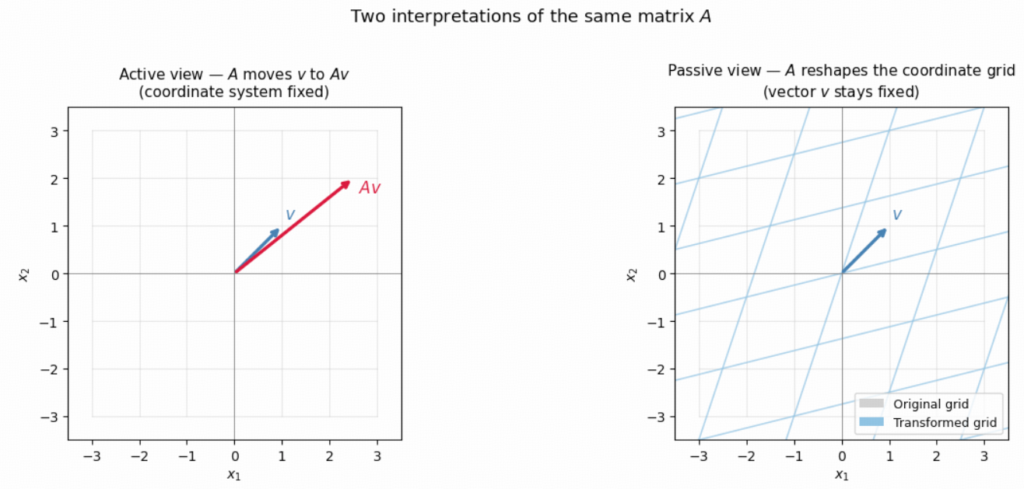
2. Columns of $A$ as Images of Basis Vectors
The most useful geometric fact:
The $j$-th column of $A$ is exactly where the $j$-th standard basis vector $e_j$ lands.
This is because $A e_j$ selects the $j$-th column. So the matrix is completely described by where it sends the axes:
$$A = \begin{bmatrix} | & | \ Ae_1 & Ae_2 \ | & | \end{bmatrix}$$
Everything else follows by linearity — any vector $v = v_1 e_1 + v_2 e_2$ maps to $Av = v_1(Ae_1) + v_2(Ae_2)$.
e1 = np.array([1.0, 0.0])
e2 = np.array([0.0, 1.0])
Ae1, Ae2 = A @ e1, A @ e2

print(f"A =\n{A}")
print(f"\nAe1 = {Ae1}  ← first column of A")
print(f"Ae2 = {Ae2}  ← second column of A")

# Verify linearity: A @ v = v[0]*Ae1 + v[1]*Ae2
v_reconstructed = v[0] * Ae1 + v[1] * Ae2
print(f"\nv = {v}")
print(f"Av via matrix multiply : {A @ v}")
print(f"Av via linear combo    : {v_reconstructed}  ✓")
A = [[2. 0.5] [0.5 1.5]] Ae1 = [2. 0.5] ← first column of A Ae2 = [0.5 1.5] ← second column of A v = [1. 1.] Av via matrix multiply : [2.5 2. ] Av via linear combo : [2.5 2. ] ✓
fig, axes = plt.subplots(1, 2, figsize=(13, 5))

for ax, (title, draw_A) in zip(axes, [
    ('Before: standard basis', False),
    ('After: columns of $A$ are new basis', True)
]):
    draw_grid(ax, A=(A if draw_A else None), color='lightgray')
    if draw_A:
        draw_arrow(ax, Ae1, color='crimson',   lw=2.5, label='$Ae_1$ (col 1)', label_offset=np.array([0.1, -0.35]))
        draw_arrow(ax, Ae2, color='darkorange', lw=2.5, label='$Ae_2$ (col 2)', label_offset=np.array([0.1,  0.1]))
        # show transformed v
        draw_arrow(ax, A @ v, color='purple', lw=2, label='$Av$', label_offset=np.array([0.1, 0.1]))
    else:
        draw_arrow(ax, e1, color='crimson',    lw=2.5, label='$e_1$', label_offset=np.array([ 0.05, -0.25]))
        draw_arrow(ax, e2, color='darkorange', lw=2.5, label='$e_2$', label_offset=np.array([-0.35,  0.1]))
        draw_arrow(ax, v,  color='purple',     lw=2,   label='$v$',   label_offset=np.array([ 0.1,   0.1]))
    style_ax(ax, title=title, xlim=(-3.5, 3.5), ylim=(-2, 4))

fig.suptitle('Columns of $A$ are the images of $e_1$ and $e_2$', fontsize=13, y=1.01)
plt.tight_layout()
plt.show()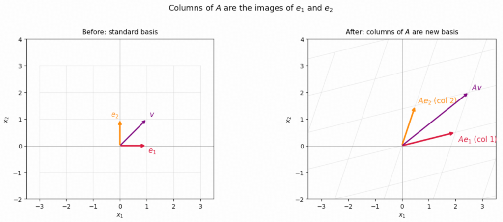
3. Non-Singular vs. Singular: Geometric Meaning
A matrix is non-singular (invertible) when its columns are linearly independent — they still span the full space after transformation. A singular matrix collapses at least one dimension.
The determinant measures the signed area (2D) or volume (nD) scaling factor:
$$\det(A) \neq 0 \iff \text{non-singular} \iff \text{no dimension is collapsed}$$
Below we compare three matrices:
- $A_1$ — non-singular, stretches and rotates
- $A_2$ — singular, collapses 2D onto a line
- $A_3$ — non-singular, reflection (det < 0, orientation flipped)
# Unit square corners (and closing point)
square = np.array([[0,1,1,0,0],
                   [0,0,1,1,0]], dtype=float)

A1 = np.array([[2.0,  0.5],   # non-singular stretch
               [0.5,  1.5]])
A2 = np.array([[1.0,  2.0],   # singular: col2 = 2*col1
               [0.5,  1.0]])
A3 = np.array([[-1.0, 0.0],   # reflection across y-axis
               [ 0.0, 1.0]])

matrices = [(A1, 'Non-singular\n$A_1$, det={:.2f}'.format(np.linalg.det(A1))),
            (A2, 'Singular\n$A_2$, det={:.2f}'.format(np.linalg.det(A2))),
            (A3, 'Non-singular (reflection)\n$A_3$, det={:.2f}'.format(np.linalg.det(A3)))]

fig, axes = plt.subplots(2, 3, figsize=(14, 9))

for col, (M, label) in enumerate(matrices):
    for row, (title_sfx, use_M) in enumerate([('Before', False), ('After', True)]):
        ax = axes[row][col]
        draw_grid(ax, A=(M if use_M else None))
        sq = M @ square if use_M else square
        ax.fill(sq[0], sq[1], alpha=0.25, color='steelblue')
        ax.plot(sq[0], sq[1], color='steelblue', lw=2)
        t = label if use_M else 'Standard basis'
        style_ax(ax, title=t, xlim=(-4,4), ylim=(-3,4))
        if use_M:
            c1, c2 = M[:, 0], M[:, 1]
            draw_arrow(ax, c1, color='crimson',    lw=2, label='col 1', label_offset=np.array([ 0.1, -0.3]))
            draw_arrow(ax, c2, color='darkorange', lw=2, label='col 2', label_offset=np.array([ 0.1,  0.1]))

axes[0][0].set_ylabel('Before', fontsize=12)
axes[1][0].set_ylabel('After $A$', fontsize=12)
fig.suptitle('Effect of non-singular vs. singular matrices on the unit square', fontsize=13)
plt.tight_layout()
plt.show()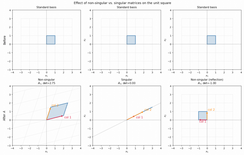
Observations:
- $A_1$ (non-singular): the square becomes a parallelogram — area changes but it remains 2D
- $A_2$ (singular): the square collapses to a line segment — all area is destroyed, the transformation is irreversible
- $A_3$ (reflection): the square flips — the negative determinant signals the orientation reversal
4. Determinant as a Volume Scaling Factor
The determinant is not just a number — it is the signed area scaling factor of the transformation.
$$\text{Area after} = |\det(A)| \times \text{Area before}$$
The sign encodes orientation: positive means the transformation preserves orientation (no reflection), negative means it reverses it.
unit_area = 1.0  # area of unit square

for M, name in [(A1,'A1 (non-singular)'), (A2,'A2 (singular)'), (A3,'A3 (reflection)')]:
    d = np.linalg.det(M)
    print(f"{name}: det = {d:+.4f},  area after = {abs(d):.4f},  orientation {'preserved' if d > 0 else 'reversed' if d < 0 else 'destroyed'}")
A1 (non-singular): det = +2.7500, area after = 2.7500, orientation preserved A2 (singular): det = +0.0000, area after = 0.0000, orientation destroyed A3 (reflection): det = -1.0000, area after = 1.0000, orientation reversed
5. SVD Decomposes the Transformation into Three Steps
The SVD $A = U \Sigma V^\top$ breaks every matrix transformation into three interpretable steps:
$$v \;\xrightarrow{V^\top}\; \text{rotate/reflect} \;\xrightarrow{\Sigma}\; \text{scale along axes} \;\xrightarrow{U}\; \text{rotate/reflect}$$
- $V^\top$ — rotates the input to align with the matrix’s natural input directions (right singular vectors)
- $\Sigma$ — stretches or compresses each axis independently by the singular values $\sigma_i$
- $U$ — rotates the result into the output orientation (left singular vectors)
Non-singular means all $\sigma_i > 0$ — every axis is scaled by a nonzero amount, so no dimension is lost.
U, s, Vt = np.linalg.svd(A1)
Sigma = np.diag(s)

print(f"A1 = U Σ Vᵀ")
print(f"\nU  =\n{np.round(U, 3)}   (rotation/reflection)")
print(f"\nΣ  = diag{np.round(s, 3)}  (scaling: σ1={s[0]:.3f}, σ2={s[1]:.3f})")
print(f"\nVᵀ =\n{np.round(Vt, 3)}   (rotation/reflection)")
print(f"\nReconstructed: U @ Σ @ Vᵀ =\n{np.round(U @ Sigma @ Vt, 6)}")
print(f"Original A1:\n{A1}  ✓")
A1 = U Σ Vᵀ U = [[-0.851 -0.526] [-0.526 0.851]] (rotation/reflection) Σ = diag[2.309 1.191] (scaling: σ1=2.309, σ2=1.191) Vᵀ = [[-0.851 -0.526] [-0.526 0.851]] (rotation/reflection) Reconstructed: U @ Σ @ Vᵀ = [[2. 0.5] [0.5 1.5]] Original A1: [[2. 0.5] [0.5 1.5]] ✓
# Visualise the four stages: v → Vᵀv → ΣVᵀv → UΣVᵀv
fig, axes = plt.subplots(1, 4, figsize=(18, 5))

# We'll track the unit circle and the standard basis arrows through each stage
theta = np.linspace(0, 2 * np.pi, 300)
circle = np.row_stack([np.cos(theta), np.sin(theta)])

stages = [
    (np.eye(2),      'Stage 0: Input space\n(unit circle + basis)'),
    (Vt,             'Stage 1: Apply $V^\\top$\n(rotate to align with singular vectors)'),
    (Sigma @ Vt,     'Stage 2: Apply $\\Sigma$\n(scale: stretch/compress)'),
    (U @ Sigma @ Vt, 'Stage 3: Apply $U$\n(rotate to output orientation = $A_1$)'),
]

for ax, (M, title) in zip(axes, stages):
    draw_grid(ax, A=M if not np.allclose(M, np.eye(2)) else None)
    c = M @ circle
    ax.plot(c[0], c[1], color='steelblue', lw=2)
    ax.fill(c[0], c[1], color='steelblue', alpha=0.15)
    draw_arrow(ax, M[:, 0], color='crimson',    lw=2)
    draw_arrow(ax, M[:, 1], color='darkorange', lw=2)
    style_ax(ax, title=title, xlim=(-3.5, 3.5), ylim=(-3.5, 3.5))

fig.suptitle('SVD decomposition: $A_1 = U\\Sigma V^\\top$ — three geometric stages', fontsize=13)
plt.tight_layout()
plt.show()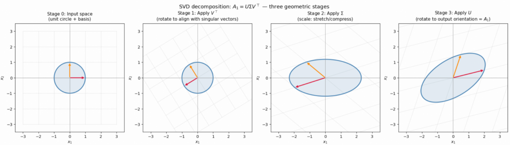
6. What Non-Singularity Guarantees
Bringing it all together:
print("=== Non-singular matrix A1 ===")
print(f"  Singular values      : {np.round(s, 4)}  (all > 0 ✓)")
print(f"  Determinant          : {np.linalg.det(A1):.4f}  (≠ 0 ✓)")
print(f"  Rank                 : {np.linalg.matrix_rank(A1)}  (= n ✓)")
print(f"  Condition number κ   : {s[0]/s[-1]:.2f}  (finite ✓)")
print(f"  Invertible           : Yes")

print()
print("=== Singular matrix A2 ===")
U2, s2, Vt2 = np.linalg.svd(A2)
print(f"  Singular values      : {np.round(s2, 6)}  (one = 0 ✗)")
print(f"  Determinant          : {np.linalg.det(A2):.6f}  (≈ 0 ✗)")
print(f"  Rank                 : {np.linalg.matrix_rank(A2)}  (< n ✗)")
print(f"  Condition number κ   : ∞")
print(f"  Invertible           : No — collapses 2D space onto a 1D line")
=== Non-singular matrix A1 === Singular values : [2.309 1.191] (all > 0 ✓) Determinant : 2.7500 (≠ 0 ✓) Rank : 2 (= n ✓) Condition number κ : 1.94 (finite ✓) Invertible : Yes === Singular matrix A2 === Singular values : [2.5 0. ] (one = 0 ✗) Determinant : 0.000000 (≈ 0 ✗) Rank : 1 (< n ✗) Condition number κ : ∞ Invertible : No — collapses 2D space onto a 1D line
Summary
| Concept | Geometric meaning |
|---|---|
| Active interpretation | $A$ moves vectors; coordinate system is fixed |
| Passive interpretation | $A$ reshapes the grid; vectors are fixed |
| Columns of $A$ | Where the standard basis vectors $e_j$ land |
| Non-singular | Columns independent → no dimension collapsed → full rank → invertible |
| $\det(A) \neq 0$ | Area/volume is scaled but not destroyed |
| $\det(A) < 0$ | Orientation is reversed (reflection component present) |
| $\det(A) = 0$ | At least one dimension is collapsed — transformation irreversible |
| SVD $A = U\Sigma V^\top$ | Rotate → scale along axes → rotate |
| All $\sigma_i > 0$ | Equivalent condition for non-singularity via SVD |
The active and passive views are two lenses on the same object. Choosing between them is a matter of which makes the problem at hand easier to reason about — not a question of which is correct.