Source: Elements of Statistical Learning, Section 2.4
This notebook walks through the theoretical framework for supervised learning: why squared error loss is natural, what EPE is, and why the optimal predictor is always the conditional expection $f(x) = \mathbb{E}[Y \mid X = x]$.
1. Setup: the prediction problem
We have:
- $X \in \mathbb{R}^p$ — a random input vector
- $Y \in \mathbb{R}$ — a random real-valued output
- Joint distribution $\Pr(X, Y)$ — we never know this fully, only observe samples from it
We want a function $f(X)$ that predicts $Y$ well.
To measure “well” we need a loss function $L(Y, f(X))$.
The most common choice is squared error loss:
$$L(Y, f(X)) = (Y – f(X))^2$$
It penalizes large errors more than small ones, is symmetric, and—crucially—is
mathematically tractable.
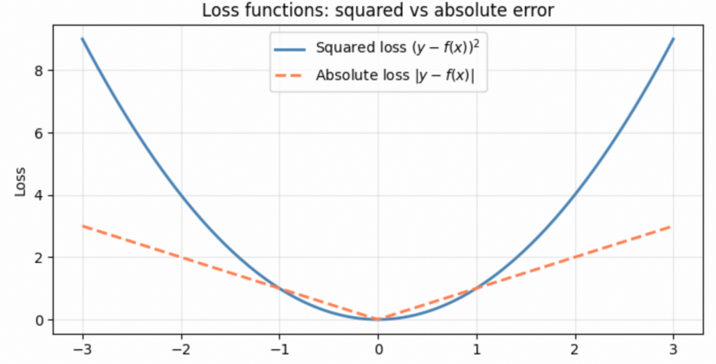
Squared loss grows quadratically — large errors are penalized much more heavily.
2. Expected Prediction Error (EPE) — Equations 2.9 & 2.10
We don’t want $f$ to do well on one specific $(x, y)$ pair.
We want it to do well on average over the whole joint distribution.
That’s the Expected Prediction Error:
$$
\text{EPE}(f) = \mathbb{E}\bigl[(Y – f(X))^2\bigr]
= \int \bigl[y – f(x)\bigr]^2 \Pr(dx,\, dy)
$$
The integral is over the full joint distribution of $(X, Y)$.
We want to find the $f$ that minimizes this.
Deep dive: what does EPE actually mean?
Your intuition is exactly right, but let’s be precise about what we’re averaging over.
The setup
We imagine a process that generates data:
Draw $(X, Y)$ from the joint distribution $\Pr(X, Y)$.
This is the same process that generates your training set and any future test point.
We never see $\Pr(X, Y)$ directly — we only observe samples from it.
EPE unpacked
$$
\text{EPE}(f) = \mathbb{E}\bigl[(Y – f(X))^2\bigr]
= \int \bigl[y – f(x)\bigr]^2 \,\Pr(dx,\, dy)
$$
The expectation is over the joint distribution of $(X, Y)$ — both inputs and outputs vary.
Think of it concretely:
- Draw a random input $X = x$ from wherever inputs come from.
- Draw the corresponding output $Y = y$ from the conditional distribution $\Pr(Y \mid X=x)$ — which may be noisy.
- Compute the squared error $(y – f(x))^2$.
- Average this over infinitely many such draws.
EPE is that long-run average squared error.
Is it “average error over a dataset”?
Almost — but with an important distinction:
| What you described | What EPE is |
|---|---|
| Average loss over a finite training set | Average loss over the true population (infinite draws) |
| $\frac{1}{n}\sum_{i=1}^n (y_i – f(x_i))^2$ — the training MSE | $\mathbb{E}_{(X,Y)}[(Y-f(X))^2]$ — the population MSE |
| Depends on which $n$ samples you happened to draw | Fixed property of $f$ and the true distribution |
The training MSE is an estimate of EPE using a finite sample.
As $n \to \infty$, training MSE $\to$ EPE (by the law of large numbers).
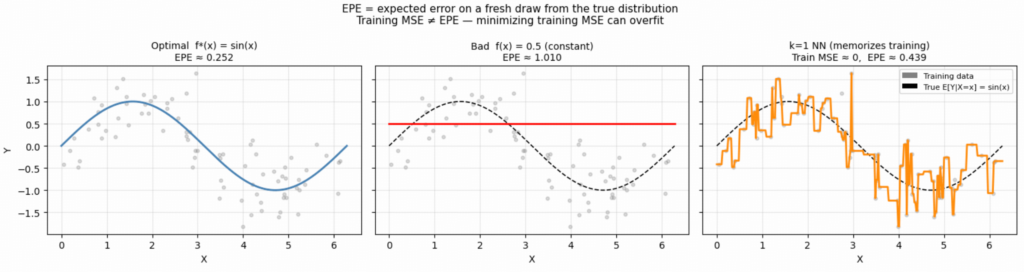
Why minimize EPE, not training MSE?
Because we care about future predictions, not memorizing the training set.
A function that memorizes training data perfectly (training MSE = 0) can have terrible EPE on new data — that’s overfitting.
The best $f$ is the one with minimum EPE — minimum expected error on a fresh draw from the same distribution.
3. Conditioning on X — Equation 2.11
The joint expectation can always be decomposed using the law of total expectation:
$$\mathbb{E}{X,Y}[\cdot] = \mathbb{E}_X\bigl[\mathbb{E}{Y|X}[\cdot \mid X]\bigr]$$
Applying this to EPE:
$$
\text{EPE}(f) = \mathbb{E}X\Bigl[\mathbb{E}{Y|X}\bigl[(Y – f(X))^2 \mid X\bigr]\Bigr]
$$
Now we have an outer expectation over $X$, and an inner expectation over $Y$ given $X$.
Key insight: the outer $\mathbb{E}_X[\cdot]$ is an average of non-negative terms.
To minimize the whole thing, it suffices to minimize the inner term pointwise —
for each fixed value of $X = x$.
4. Pointwise minimization — Equation 2.12
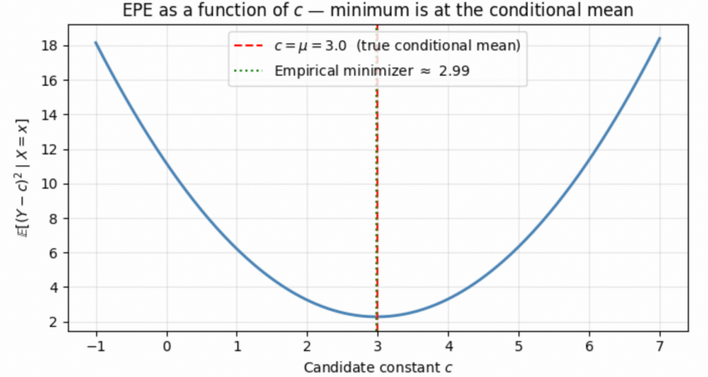
Fix $X = x$. We ask: what constant $c$ minimizes
$$\mathbb{E}_{Y|X}\bigl[(Y – c)^2 \mid X = x\bigr]\,?$$
This is a function of $c$ alone. Take the derivative and set to zero:
$$
\frac{d}{dc}\,\mathbb{E}[(Y-c)^2 \mid X=x]
= \mathbb{E}\bigl[2(Y-c)(-1) \mid X=x\bigr]
= -2\,\mathbb{E}[Y – c \mid X=x] = 0
$$
$$\Rightarrow\quad \mathbb{E}[Y \mid X=x] = c$$
So the minimizing constant at each point $x$ is exactly the conditional mean of $Y$ given $X=x$.
Therefore:
$$
f(x) = \mathbb{E}[Y \mid X = x] \qquad \text{(Eq. 2.13)}
$$
This is called the regression function.
5. Bias-Variance decomposition: why the minimum is the conditional mean
There’s a cleaner algebraic way to see the same result.
Add and subtract $\mathbb{E}[Y \mid X=x]$, letting $\mu(x) = \mathbb{E}[Y \mid X=x]$:
$$
(Y – c)^2 = \bigl[(Y – \mu(x)) + (\mu(x) – c)\bigr]^2
= (Y – \mu(x))^2 + 2(Y – \mu(x))(\mu(x) – c) + (\mu(x) – c)^2
$$
Taking $\mathbb{E}[\cdot \mid X=x]$, the cross term vanishes because $\mathbb{E}[Y – \mu(x) \mid X=x] = 0$:
$$
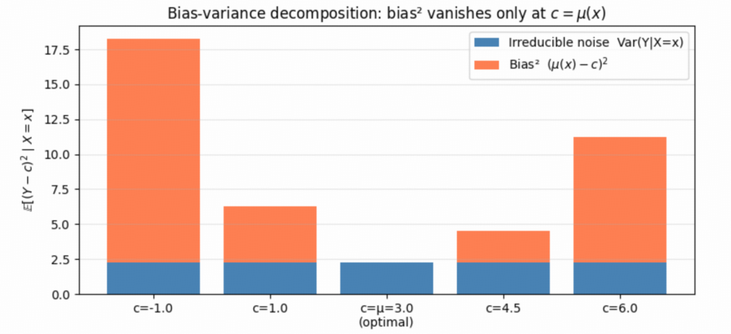
\mathbb{E}[(Y-c)^2 \mid X=x] = \underbrace{\text{Var}(Y \mid X=x)}{\text{irreducible noise}} + \underbrace{(\mu(x) – c)^2}{\text{bias}^2}
$$
The first term is fixed — no choice of $c$ can remove the inherent randomness of $Y$.
The second term is zero exactly when $c = \mu(x) = \mathbb{E}[Y \mid X=x]$.
This is the bias-variance decomposition in its simplest form.
6. The full picture: putting it together
| Step | What we do | Result |
|---|---|---|
| Define problem | Want $f$ to predict $Y$ from $X$ | Need a loss function |
| Choose loss | Squared error $(Y – f(X))^2$ | Tractable, penalizes large errors |
| Define criterion | $\text{EPE}(f) = \mathbb{E}[(Y-f(X))^2]$ | Global average loss |
| Condition on $X$ | Law of total expectation | $\text{EPE} = \mathbb{E}X[\mathbb{E}{Y |
| Minimize pointwise | At each $x$, minimize over constant $c$ | $c^* = \mathbb{E}[Y \mid X=x]$ |
| Conclusion | Optimal predictor | $f(x) = \mathbb{E}[Y \mid X=x]$ |
The regression function $f(x) = \mathbb{E}[Y \mid X=x]$ is the theoretical gold standard.
Every regression method (linear regression, kNN, neural networks, gradient boosting)
is an attempt to approximate this function from finite training data.
7. Why nearest-neighbor methods follow from this
The text ends by saying nearest-neighbor methods try to directly implement this recipe.
Here’s the idea:
$$f(x) = \mathbb{E}[Y \mid X = x] \approx \frac{1}{k} \sum_{x_i \in N_k(x)} y_i$$
where $N_k(x)$ is the set of $k$ training points closest to $x$.
This approximation relies on two hopes:
- Averaging approximates expectation (law of large numbers)
- Nearby points $x_i \approx x$, so conditioning on $X = x_i$ ≈ conditioning on $X = x$
Both hopes fail in high dimensions (the curse of dimensionality) — but that’s ESL Section 2.5.
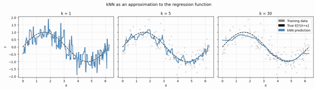
k=1: low bias, high variance (wiggly)
k=30: high bias, low variance (smooth but misses local structure)
The true E[Y|X=x] = sin(x) is what all k choices try to approximate.