This notebook builds a complete understanding of GBDT from the ground up:
- Decision trees as weak learners
- Ensemble methods: bagging vs. boosting
- The gradient boosting algorithm — mathematical derivation
- GBDT from scratch (regression)
- Loss functions and their gradients
- Scikit-learn implementation (regression + classification)
- Hyperparameter effects
- Feature importance
- Overfitting and regularisation
- Random Forest vs. GBDT comparison
import numpy as np
import matplotlib.pyplot as plt
import matplotlib.gridspec as gridspec
from sklearn.tree import DecisionTreeRegressor, DecisionTreeClassifier, plot_tree
from sklearn.ensemble import GradientBoostingRegressor, GradientBoostingClassifier, RandomForestClassifier
from sklearn.datasets import make_regression, make_classification, make_moons
from sklearn.model_selection import train_test_split
from sklearn.metrics import mean_squared_error, accuracy_score
from sklearn.preprocessing import StandardScaler
import warnings
warnings.filterwarnings('ignore')

rng = np.random.default_rng(42)
plt.rcParams['figure.dpi'] = 100
1. Decision Trees: The Weak Learner
GBDT builds an ensemble of decision trees. Each tree partitions the feature space into rectangular regions and predicts a constant value in each region.
A single deep tree overfits; a single shallow tree (a stump) underfits. GBDT uses many shallow trees — deliberately weak — and combines them sequentially.
Why shallow trees?
- Low variance: they don’t chase noise
- Fast to train
- Their errors are systematic (high bias), which subsequent trees can correct
# Generate a simple 1D regression problem
np.random.seed(42)
X_1d = np.sort(np.random.uniform(0, 10, 120))
y_1d = np.sin(X_1d) + 0.3 * np.random.randn(120)
X_1d = X_1d.reshape(-1, 1)

x_plot = np.linspace(0, 10, 500).reshape(-1, 1)

fig, axes = plt.subplots(1, 3, figsize=(15, 4))
depths = [1, 3, 10]
titles = ['Stump (depth=1)\nHigh bias, low variance',
          'Shallow tree (depth=3)\nBetter balance',
          'Deep tree (depth=10)\nLow bias, high variance']

for ax, d, title in zip(axes, depths, titles):
    tree = DecisionTreeRegressor(max_depth=d, random_state=42)
    tree.fit(X_1d, y_1d)
    ax.scatter(X_1d, y_1d, s=15, alpha=0.5, color='gray', label='Data')
    ax.plot(x_plot, tree.predict(x_plot), color='crimson', lw=2, label=f'Tree (depth={d})')
    ax.plot(x_plot, np.sin(x_plot), 'k--', lw=1.5, alpha=0.5, label='True signal')
    train_mse = mean_squared_error(y_1d, tree.predict(X_1d))
    ax.set_title(f'{title}\nTrain MSE={train_mse:.3f}')
    ax.legend(fontsize=8)
    ax.set_xlabel('x'); ax.set_ylabel('y')

plt.suptitle('Single decision trees: bias-variance trade-off', fontsize=13)
plt.tight_layout()
plt.show()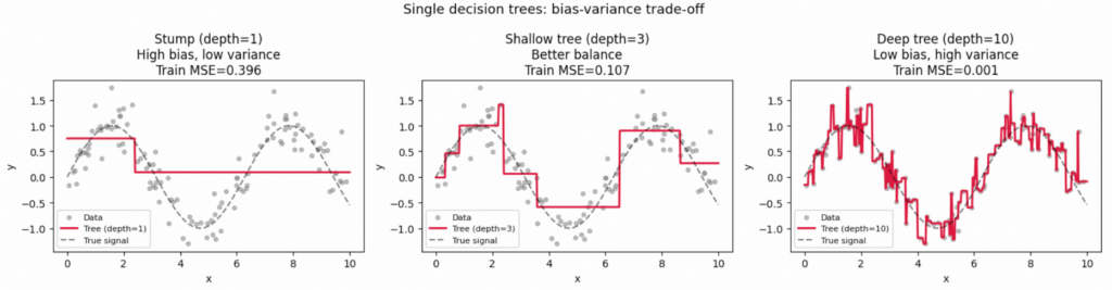
2. Ensemble Methods: Bagging vs. Boosting
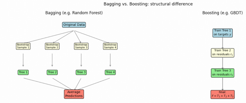
Both methods combine many weak learners, but in fundamentally different ways:
| Bagging | Boosting | |
|---|---|---|
| Training order | Parallel (independent) | Sequential (each depends on previous) |
| How errors are addressed | Averaging reduces variance | Each model corrects prior errors |
| Data sampling | Bootstrap resamples | Reweights or fits residuals |
| Typical depth | Deep trees | Shallow trees (stumps) |
| Risk | Low variance, can still have bias | Low bias, can overfit |
| Example | Random Forest | GBDT, AdaBoost |
The key boosting idea: each new model is trained not on the original targets $y$, but on the errors of the current ensemble. The ensemble improves iteratively.
fig, axes = plt.subplots(1, 2, figsize=(13, 5))

# ── Bagging diagram ────────────────────────────────────────────────────────
ax = axes[0]
ax.set_xlim(0, 10); ax.set_ylim(0, 8); ax.axis('off')
ax.set_title('Bagging (e.g. Random Forest)', fontsize=12, pad=10)

ax.text(5, 7.3, 'Original Data', ha='center', fontsize=10,
        bbox=dict(boxstyle='round', facecolor='lightblue'))
for i, x in enumerate([1.5, 3.5, 5.5, 7.5, 9.0]):
    if i < 4:
        ax.annotate('', xy=(x, 5.8), xytext=(5, 6.9),
                    arrowprops=dict(arrowstyle='->', color='gray'))
        ax.text(x, 5.4, f'Bootstrap\nSample {i+1}', ha='center', fontsize=8,
                bbox=dict(boxstyle='round', facecolor='lightyellow'))
        ax.annotate('', xy=(x, 3.8), xytext=(x, 5.0),
                    arrowprops=dict(arrowstyle='->', color='gray'))
        ax.text(x, 3.3, f'Tree {i+1}', ha='center', fontsize=9,
                bbox=dict(boxstyle='round', facecolor='lightgreen'))
        ax.annotate('', xy=(5, 1.8), xytext=(x, 2.9),
                    arrowprops=dict(arrowstyle='->', color='gray'))
ax.text(5, 1.3, 'Average\nPredictions', ha='center', fontsize=10,
        bbox=dict(boxstyle='round', facecolor='salmon'))

# ── Boosting diagram ───────────────────────────────────────────────────────
ax = axes[1]
ax.set_xlim(0, 10); ax.set_ylim(0, 8); ax.axis('off')
ax.set_title('Boosting (e.g. GBDT)', fontsize=12, pad=10)

steps = ['Train Tree 1\non targets $y$',
         'Train Tree 2\non residuals $r_1$',
         'Train Tree 3\non residuals $r_2$',
         'Final:\n$F = T_1 + T_2 + T_3$']
colors = ['lightblue', 'lightyellow', 'lightgreen', 'salmon']
ys = [6.5, 4.8, 3.1, 1.3]
for i, (step, c, y) in enumerate(zip(steps, colors, ys)):
    ax.text(5, y, step, ha='center', fontsize=9,
            bbox=dict(boxstyle='round', facecolor=c))
    if i < len(steps) - 1:
        ax.annotate('', xy=(5, ys[i+1]+0.45), xytext=(5, y-0.1),
                    arrowprops=dict(arrowstyle='->', color='gray', lw=1.5))

plt.suptitle('Bagging vs. Boosting: structural difference', fontsize=13)
plt.tight_layout()
plt.show()
3. The Gradient Boosting Algorithm
Gradient boosting frames boosting as gradient descent in function space.
Setup
We want to find a function $F(x)$ that minimises the expected loss:
$$\mathcal{L} = \sum_{i=1}^{n} L(y_i, F(x_i))$$
Instead of optimising over parameters, we optimise over functions by taking gradient steps. At each step $m$, we ask:
In which direction should we nudge $F$ at each training point to most reduce the loss?
The answer is the negative gradient of the loss with respect to $F(x_i)$:
$$r_{im} = -\left[\frac{\partial L(y_i,\, F(x_i))}{\partial F(x_i)}\right]{F = F{m-1}}$$
These $r_{im}$ are called pseudo-residuals.
Algorithm
Initialise: $F_0(x) = \arg\min_\gamma \sum_{i} L(y_i, \gamma)$ (a constant — e.g. the mean for MSE)
For $m = 1, 2, \ldots, M$:
- Compute pseudo-residuals: $r_{im} = -\frac{\partial L(y_i, F_{m-1}(x_i))}{\partial F_{m-1}(x_i)}$
- Fit a tree $h_m(x)$ to ${(x_i, r_{im})}$
- Find the optimal step size: $\gamma_m = \arg\min_\gamma \sum_i L(y_i,\, F_{m-1}(x_i) + \gamma\, h_m(x_i))$
- Update: $F_m(x) = F_{m-1}(x) + \nu \cdot \gamma_m \cdot h_m(x)$
where $\nu \in (0,1]$ is the learning rate (shrinkage).
For MSE loss
$$L(y, F) = \tfrac{1}{2}(y – F)^2 \implies r_{im} = y_i – F_{m-1}(x_i)$$
The pseudo-residuals are exactly the ordinary residuals. Each tree fits the errors left by the current ensemble.
4. GBDT from Scratch (Regression, MSE Loss)
We implement the algorithm step by step to see every moving part.
class GBDTRegressor:
    """
    Gradient Boosted Decision Trees for regression with MSE loss.
    Pseudo-residuals = ordinary residuals (y - F).
    """
    def __init__(self, n_estimators=100, learning_rate=0.1, max_depth=3):
        self.n_estimators  = n_estimators
        self.learning_rate = learning_rate
        self.max_depth     = max_depth
        self.trees_         = []
        self.F0_            = None     # initial constant prediction

    def fit(self, X, y):
        # Step 0: initialise with the mean
        self.F0_ = np.mean(y)
        F = np.full(len(y), self.F0_)

        for m in range(self.n_estimators):
            # Step 1: compute pseudo-residuals (negative gradient of MSE)
            residuals = y - F

            # Step 2: fit a tree to the pseudo-residuals
            tree = DecisionTreeRegressor(max_depth=self.max_depth, random_state=m)
            tree.fit(X, residuals)
            self.trees_.append(tree)

            # Step 3 & 4: update prediction
            F += self.learning_rate * tree.predict(X)

        return self

    def predict(self, X):
        F = np.full(len(X), self.F0_)
        for tree in self.trees_:
            F += self.learning_rate * tree.predict(X)
        return F

    def staged_predict(self, X):
        """Yield predictions after each boosting round."""
        F = np.full(len(X), self.F0_)
        yield F.copy()
        for tree in self.trees_:
            F += self.learning_rate * tree.predict(X)
            yield F.copy()
# Train and visualise the sequential build-up
gbdt_scratch = GBDTRegressor(n_estimators=50, learning_rate=0.3, max_depth=2)
gbdt_scratch.fit(X_1d, y_1d)
x_plot = np.linspace(0, 10, 500).reshape(-1, 1)
stages = [1, 3, 8, 20, 50]
predictions = list(gbdt_scratch.staged_predict(x_plot))
fig, axes = plt.subplots(1, len(stages), figsize=(18, 4), sharey=True)
for ax, m in zip(axes, stages):
ax.scatter(X_1d, y_1d, s=12, alpha=0.4, color='gray')
ax.plot(x_plot, np.sin(x_plot), 'k--', lw=1.5, alpha=0.5, label='True')
ax.plot(x_plot, predictions[m], color='crimson', lw=2, label=f'm={m}')
train_mse = mean_squared_error(y_1d, list(gbdt_scratch.staged_predict(X_1d))[m])
ax.set_title(f'{m} tree{"s" if m>1 else ""}\nMSE={train_mse:.4f}')
ax.legend(fontsize=8)
ax.set_xlabel('x')
axes[0].set_ylabel('y')
plt.suptitle('GBDT from scratch: ensemble fit after $m$ trees (lr=0.3, depth=2)', fontsize=13)
plt.tight_layout()
plt.show()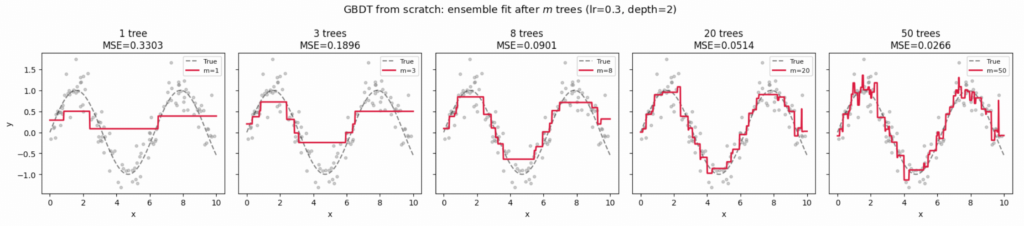
# Show the residuals being fitted at each step
fig, axes = plt.subplots(1, 4, figsize=(16, 4))
F = np.full(len(X_1d), gbdt_scratch.F0_)

for ax, m in zip(axes, [0, 1, 2, 4]):
    for i in range(m):
        F += gbdt_scratch.learning_rate * gbdt_scratch.trees_[i].predict(X_1d)
    residuals = y_1d - F
    ax.scatter(X_1d, residuals, s=12, alpha=0.5, color='steelblue')
    ax.axhline(0, color='crimson', lw=1.5, linestyle='--')
    ax.set_title(f'Residuals after {m} tree{"s" if m!=1 else ""}')
    ax.set_xlabel('x')
    rss = np.sum(residuals**2)
    ax.text(0.05, 0.95, f'RSS={rss:.2f}', transform=ax.transAxes, va='top', fontsize=9,
            bbox=dict(boxstyle='round', facecolor='wheat', alpha=0.7))
    F = np.full(len(X_1d), gbdt_scratch.F0_)  # reset for next panel

axes[0].set_ylabel('Residual')
plt.suptitle('Pseudo-residuals shrink as more trees are added', fontsize=13)
plt.tight_layout()
plt.show()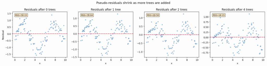
5. Loss Functions and Their Gradients
The choice of loss function determines what the pseudo-residuals represent.
| Task | Loss $L(y, F)$ | Pseudo-residual $r = -\partial L / \partial F$ |
|---|---|---|
| Regression (MSE) | $\frac{1}{2}(y-F)^2$ | $y – F$ |
| Regression (MAE) | $ | y – F |
| Regression (Huber) | Quadratic near 0, linear in tails | Clipped residuals |
| Classification | $\log(1 + e^{-yF})$ (log-loss) | $y – \sigma(F)$ where $\sigma$ is sigmoid |
The gradient of MAE is just the sign — the tree fits the direction of the error, not the magnitude. This makes MAE-based GBDT robust to outliers.
F_vals = np.linspace(-3, 3, 300)
y_true = 1.0

mse_loss    = 0.5 * (y_true - F_vals)**2
mse_grad    = -(y_true - F_vals)          # negative gradient = residual
mae_loss    = np.abs(y_true - F_vals)
mae_grad    = -np.sign(y_true - F_vals)

# Huber
delta = 1.0
diff = y_true - F_vals
huber_loss = np.where(np.abs(diff) <= delta,
                      0.5 * diff**2,
                      delta * (np.abs(diff) - 0.5 * delta))
huber_grad = np.where(np.abs(diff) <= delta, -diff, -delta * np.sign(diff))

fig, axes = plt.subplots(1, 2, figsize=(13, 4))

ax = axes[0]
ax.plot(F_vals, mse_loss,   label='MSE',   color='steelblue', lw=2)
ax.plot(F_vals, mae_loss,   label='MAE',   color='crimson',   lw=2)
ax.plot(F_vals, huber_loss, label='Huber', color='green',     lw=2)
ax.axvline(y_true, color='gray', lw=1, linestyle='--', label=f'y={y_true}')
ax.set_xlabel('F(x)'); ax.set_ylabel('Loss'); ax.set_title('Loss functions')
ax.legend(); ax.grid(True, alpha=0.3)

ax = axes[1]
ax.plot(F_vals, mse_grad,   label='MSE pseudo-residual',   color='steelblue', lw=2)
ax.plot(F_vals, mae_grad,   label='MAE pseudo-residual',   color='crimson',   lw=2)
ax.plot(F_vals, huber_grad, label='Huber pseudo-residual', color='green',     lw=2)
ax.axvline(y_true, color='gray', lw=1, linestyle='--')
ax.axhline(0, color='gray', lw=0.7)
ax.set_xlabel('F(x)'); ax.set_ylabel('Pseudo-residual')
ax.set_title('Pseudo-residuals = negative gradient')
ax.legend(); ax.grid(True, alpha=0.3)

plt.suptitle('Loss functions and their pseudo-residuals (y=1.0)', fontsize=13)
plt.tight_layout()
plt.show()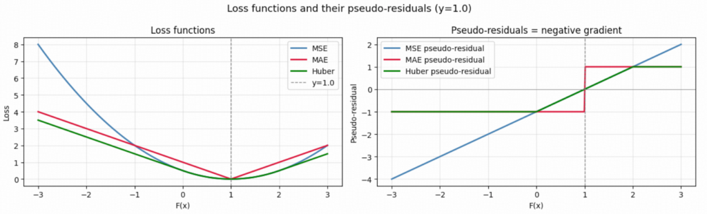
6. Scikit-learn Implementation
6a. Regression
X_reg, y_reg = make_regression(n_samples=500, n_features=10, noise=20, random_state=42)
X_tr, X_te, y_tr, y_te = train_test_split(X_reg, y_reg, test_size=0.2, random_state=42)

gbr = GradientBoostingRegressor(
    n_estimators=200,
    learning_rate=0.1,
    max_depth=3,
    subsample=0.8,       # stochastic gradient boosting
    random_state=42
)
gbr.fit(X_tr, y_tr)

# Staged test error
train_errors = [mean_squared_error(y_tr, pred) for pred in gbr.staged_predict(X_tr)]
test_errors  = [mean_squared_error(y_te, pred) for pred in gbr.staged_predict(X_te)]

fig, axes = plt.subplots(1, 2, figsize=(13, 4))

ax = axes[0]
ax.plot(train_errors, label='Train MSE', color='steelblue', lw=2)
ax.plot(test_errors,  label='Test MSE',  color='crimson',   lw=2)
ax.set_xlabel('Number of trees'); ax.set_ylabel('MSE')
ax.set_title('Learning curve: MSE vs. number of trees')
ax.legend(); ax.grid(True, alpha=0.3)

ax = axes[1]
y_pred = gbr.predict(X_te)
ax.scatter(y_te, y_pred, alpha=0.4, s=20, color='steelblue')
mn, mx = min(y_te.min(), y_pred.min()), max(y_te.max(), y_pred.max())
ax.plot([mn, mx], [mn, mx], 'k--', lw=1.5, label='Perfect prediction')
ax.set_xlabel('True'); ax.set_ylabel('Predicted')
ax.set_title(f'Predicted vs. True (Test MSE={test_errors[-1]:.1f})')
ax.legend(); ax.grid(True, alpha=0.3)

plt.suptitle('GradientBoostingRegressor — scikit-learn', fontsize=13)
plt.tight_layout()
plt.show()

print(f"Final Train MSE : {train_errors[-1]:.2f}")
print(f"Final Test MSE  : {test_errors[-1]:.2f}")
6b. Classification
For binary classification GBDT uses log-loss (cross-entropy). The model outputs a log-odds score $F(x)$, converted to a probability via the sigmoid:
$$P(y=1 \mid x) = \sigma(F(x)) = \frac{1}{1 + e^{-F(x)}}$$
The pseudo-residuals become: $r_i = y_i – \sigma(F(x_i))$ — the difference between the true label and the predicted probability.
X_moons, y_moons = make_moons(n_samples=600, noise=0.25, random_state=42)
X_tr_c, X_te_c, y_tr_c, y_te_c = train_test_split(X_moons, y_moons, test_size=0.25, random_state=42)

gbc = GradientBoostingClassifier(n_estimators=200, learning_rate=0.1,
                                  max_depth=3, random_state=42)
gbc.fit(X_tr_c, y_tr_c)

# Decision boundary
def plot_decision_boundary(ax, model, X, y, title):
    h = 0.03
    x_min, x_max = X[:,0].min()-0.5, X[:,0].max()+0.5
    y_min, y_max = X[:,1].min()-0.5, X[:,1].max()+0.5
    xx, yy = np.meshgrid(np.arange(x_min, x_max, h),
                         np.arange(y_min, y_max, h))
    Z = model.predict_proba(np.c_[xx.ravel(), yy.ravel()])[:,1]
    Z = Z.reshape(xx.shape)
    ax.contourf(xx, yy, Z, alpha=0.3, cmap='RdBu_r', levels=20)
    ax.contour(xx, yy, Z, levels=[0.5], colors='black', linewidths=1.5)
    ax.scatter(X[:,0], X[:,1], c=y, cmap='RdBu_r', s=20, edgecolors='k', lw=0.3)
    acc = accuracy_score(y, model.predict(X))
    ax.set_title(f'{title}\nAccuracy={acc:.3f}')

fig, axes = plt.subplots(1, 3, figsize=(15, 4))

# Show progression
for ax, n in zip(axes, [5, 30, 200]):
    m = GradientBoostingClassifier(n_estimators=n, learning_rate=0.1,
                                    max_depth=3, random_state=42)
    m.fit(X_tr_c, y_tr_c)
    plot_decision_boundary(ax, m, X_te_c, y_te_c, f'{n} trees')

plt.suptitle('GBDT classification on moons dataset: decision boundary evolution', fontsize=13)
plt.tight_layout()
plt.show()
7. Hyperparameter Effects
GBDT has several important hyperparameters:
| Parameter | Effect |
|---|---|
n_estimators | More trees → lower bias, risk of overfitting |
learning_rate | Smaller → need more trees, but generalises better |
max_depth | Controls complexity of each tree |
subsample | Fraction of data per tree — reduces variance (stochastic GB) |
min_samples_leaf | Smooths leaf predictions, reduces overfitting |
The learning rate–n_estimators trade-off: a small learning rate requires many trees to achieve the same training loss, but typically yields better generalisation. These two are always tuned together.
fig, axes = plt.subplots(2, 2, figsize=(13, 10))

# ── 1. Learning rate ────────────────────────────────────────────────────────
ax = axes[0][0]
for lr in [0.01, 0.05, 0.1, 0.5]:
    m = GradientBoostingRegressor(n_estimators=200, learning_rate=lr,
                                   max_depth=3, random_state=42)
    m.fit(X_tr, y_tr)
    te = [mean_squared_error(y_te, p) for p in m.staged_predict(X_te)]
    ax.plot(te, label=f'lr={lr}', lw=1.8)
ax.set_xlabel('n_estimators'); ax.set_ylabel('Test MSE')
ax.set_title('Effect of learning rate'); ax.legend(); ax.grid(True, alpha=0.3)

# ── 2. Tree depth ──────────────────────────────────────────────────────────
ax = axes[0][1]
for d in [1, 2, 3, 5, 8]:
    m = GradientBoostingRegressor(n_estimators=200, learning_rate=0.1,
                                   max_depth=d, random_state=42)
    m.fit(X_tr, y_tr)
    te = [mean_squared_error(y_te, p) for p in m.staged_predict(X_te)]
    ax.plot(te, label=f'depth={d}', lw=1.8)
ax.set_xlabel('n_estimators'); ax.set_ylabel('Test MSE')
ax.set_title('Effect of tree depth'); ax.legend(); ax.grid(True, alpha=0.3)

# ── 3. Subsample ───────────────────────────────────────────────────────────
ax = axes[1][0]
for ss in [0.3, 0.5, 0.8, 1.0]:
    m = GradientBoostingRegressor(n_estimators=200, learning_rate=0.1,
                                   max_depth=3, subsample=ss, random_state=42)
    m.fit(X_tr, y_tr)
    te = [mean_squared_error(y_te, p) for p in m.staged_predict(X_te)]
    ax.plot(te, label=f'subsample={ss}', lw=1.8)
ax.set_xlabel('n_estimators'); ax.set_ylabel('Test MSE')
ax.set_title('Effect of subsample (stochastic GB)'); ax.legend(); ax.grid(True, alpha=0.3)

# ── 4. lr × n_estimators trade-off ─────────────────────────────────────────
ax = axes[1][1]
configs = [(0.5, 40), (0.1, 200), (0.05, 400), (0.01, 2000)]
results = []
for lr, n in configs:
    m = GradientBoostingRegressor(n_estimators=n, learning_rate=lr,
                                   max_depth=3, random_state=42)
    m.fit(X_tr, y_tr)
    results.append(mean_squared_error(y_te, m.predict(X_te)))
labels = [f'lr={lr}, n={n}' for lr, n in configs]
bars = ax.bar(labels, results, color=['steelblue','darkorange','green','crimson'], alpha=0.8)
ax.set_ylabel('Test MSE')
ax.set_title('lr × n_estimators trade-off\n(same approximate total "work")')
ax.tick_params(axis='x', rotation=15)
for bar, val in zip(bars, results):
    ax.text(bar.get_x() + bar.get_width()/2, bar.get_height() + 5,
            f'{val:.0f}', ha='center', fontsize=9)
ax.grid(True, alpha=0.3, axis='y')

plt.suptitle('Hyperparameter effects on test MSE', fontsize=13)
plt.tight_layout()
plt.show()
8. Feature Importance
GBDT computes feature importance as the total reduction in loss (impurity) due to splits on each feature, summed across all trees:
$$\text{importance}(f) = \sum_{m=1}^{M} \sum_{\text{nodes } t \in h_m \text{ that split on } f} \Delta L_t$$
where $\Delta L_t$ is the reduction in the split criterion at node $t$.
Limitations: this measure favours high-cardinality features and can be misleading when features are correlated. Permutation importance is a more reliable alternative.
from sklearn.inspection import permutation_importance

feature_names = [f'Feature {i+1}' for i in range(X_reg.shape[1])]

# Built-in impurity importance
imp_builtin = gbr.feature_importances_

# Permutation importance (on test set)
perm = permutation_importance(gbr, X_te, y_te, n_repeats=20, random_state=42)
imp_perm = perm.importances_mean

idx_b = np.argsort(imp_builtin)[::-1]
idx_p = np.argsort(imp_perm)[::-1]

fig, axes = plt.subplots(1, 2, figsize=(13, 4))

ax = axes[0]
ax.bar(range(len(idx_b)), imp_builtin[idx_b], color='steelblue', alpha=0.8)
ax.set_xticks(range(len(idx_b)))
ax.set_xticklabels([feature_names[i] for i in idx_b], rotation=45, ha='right')
ax.set_title('Built-in impurity-based importance'); ax.set_ylabel('Importance')
ax.grid(True, alpha=0.3, axis='y')

ax = axes[1]
ax.bar(range(len(idx_p)), imp_perm[idx_p], color='crimson', alpha=0.8,
       yerr=perm.importances_std[idx_p], capsize=4)
ax.set_xticks(range(len(idx_p)))
ax.set_xticklabels([feature_names[i] for i in idx_p], rotation=45, ha='right')
ax.set_title('Permutation importance (test set)'); ax.set_ylabel('Mean MSE increase')
ax.grid(True, alpha=0.3, axis='y')

plt.suptitle('Feature importance: impurity-based vs. permutation', fontsize=13)
plt.tight_layout()
plt.show()
9. Overfitting and Regularisation
GBDT can overfit, especially with:
- Too many trees (
n_estimatorstoo large without shrinkage) - Too large a learning rate
- Too deep trees (
max_depth)
Regularisation strategies:
| Strategy | Parameter | Mechanism |
|---|---|---|
| Shrinkage | learning_rate | Scales each tree’s contribution down |
| Stochastic GB | subsample < 1 | Trains each tree on a random subsample |
| Tree constraints | max_depth, min_samples_leaf | Limits individual tree complexity |
| Early stopping | n_iter_no_change | Halts when validation loss stops improving |
# Demonstrate overfitting then early stopping
fig, axes = plt.subplots(1, 2, figsize=(13, 4))

# ── Overfitting: high lr, deep trees ──────────────────────────────────────
ax = axes[0]
m_overfit = GradientBoostingRegressor(n_estimators=500, learning_rate=0.5,
                                       max_depth=6, random_state=42)
m_overfit.fit(X_tr, y_tr)
tr_e = [mean_squared_error(y_tr, p) for p in m_overfit.staged_predict(X_tr)]
te_e = [mean_squared_error(y_te, p) for p in m_overfit.staged_predict(X_te)]
best_n = np.argmin(te_e)
ax.plot(tr_e, label='Train', color='steelblue', lw=2)
ax.plot(te_e, label='Test',  color='crimson',   lw=2)
ax.axvline(best_n, color='green', lw=2, linestyle='--',
           label=f'Best test @ n={best_n}')
ax.set_xlabel('n_estimators'); ax.set_ylabel('MSE')
ax.set_title('Overfitting: high lr (0.5), deep trees (depth=6)')
ax.legend(); ax.grid(True, alpha=0.3)

# ── Early stopping ─────────────────────────────────────────────────────────
ax = axes[1]
m_es = GradientBoostingRegressor(
    n_estimators=500,
    learning_rate=0.5,
    max_depth=6,
    n_iter_no_change=15,   # stop if no improvement for 15 rounds
    validation_fraction=0.15,
    random_state=42
)
m_es.fit(X_tr, y_tr)
te_e2 = [mean_squared_error(y_te, p) for p in m_es.staged_predict(X_te)]
ax.plot(te_e,  label='Without early stopping', color='crimson',   lw=2, alpha=0.7)
ax.plot(te_e2, label='With early stopping',    color='steelblue', lw=2)
ax.axvline(m_es.n_estimators_ - 1, color='green', lw=2, linestyle='--',
           label=f'Stopped @ n={m_es.n_estimators_}')
ax.set_xlabel('n_estimators'); ax.set_ylabel('Test MSE')
ax.set_title('Early stopping prevents overfitting')
ax.legend(); ax.grid(True, alpha=0.3)

plt.suptitle('Overfitting and early stopping in GBDT', fontsize=13)
plt.tight_layout()
plt.show()

print(f"Without early stopping — final test MSE : {te_e[-1]:.2f}  ({len(te_e)} trees)")
print(f"With early stopping    — final test MSE : {te_e2[-1]:.2f}  ({m_es.n_estimators_} trees)")
10. Random Forest vs. GBDT
Both are tree ensembles but operate on different principles. Neither is universally better — the choice depends on the problem.
from sklearn.ensemble import RandomForestClassifier

X_cl, y_cl = make_classification(n_samples=1000, n_features=20, n_informative=10,
                                   n_redundant=5, random_state=42)
X_tr2, X_te2, y_tr2, y_te2 = train_test_split(X_cl, y_cl, test_size=0.25, random_state=42)

n_range = [1, 5, 10, 20, 50, 100, 200]
rf_scores, gbdt_scores = [], []

for n in n_range:
    rf = RandomForestClassifier(n_estimators=n, random_state=42)
    rf.fit(X_tr2, y_tr2)
    rf_scores.append(accuracy_score(y_te2, rf.predict(X_te2)))

    gb = GradientBoostingClassifier(n_estimators=n, learning_rate=0.1,
                                     max_depth=3, random_state=42)
    gb.fit(X_tr2, y_tr2)
    gbdt_scores.append(accuracy_score(y_te2, gb.predict(X_te2)))

fig, axes = plt.subplots(1, 2, figsize=(13, 4))

ax = axes[0]
ax.plot(n_range, rf_scores,   'o-', label='Random Forest', color='steelblue', lw=2)
ax.plot(n_range, gbdt_scores, 's-', label='GBDT',          color='crimson',   lw=2)
ax.set_xlabel('n_estimators'); ax.set_ylabel('Test Accuracy')
ax.set_title('Accuracy vs. number of trees')
ax.legend(); ax.grid(True, alpha=0.3)

# Side-by-side comparison on moons
ax = axes[1]
models = [
    ('Random Forest',  RandomForestClassifier(n_estimators=200, random_state=42)),
    ('GBDT',           GradientBoostingClassifier(n_estimators=200, learning_rate=0.1,
                                                   max_depth=3, random_state=42)),
]
for name, mdl in models:
    mdl.fit(X_tr_c, y_tr_c)
accs = [accuracy_score(y_te_c, m.predict(X_te_c)) for _, m in models]
names = [n for n, _ in models]
bars = ax.bar(names, accs, color=['steelblue', 'crimson'], alpha=0.8)
for bar, acc in zip(bars, accs):
    ax.text(bar.get_x() + bar.get_width()/2, bar.get_height() - 0.02,
            f'{acc:.3f}', ha='center', va='top', color='white', fontweight='bold')
ax.set_ylim(0.8, 1.0); ax.set_ylabel('Test Accuracy')
ax.set_title('Accuracy on moons dataset (n=200 trees)')
ax.grid(True, alpha=0.3, axis='y')

plt.suptitle('Random Forest vs. GBDT', fontsize=13)
plt.tight_layout()
plt.show()

print("\nRandom Forest vs. GBDT — summary:")
print(f"{'Property':<30} {'Random Forest':<22} {'GBDT'}")
print("-" * 70)
rows = [
    ('Training strategy',    'Parallel (independent)', 'Sequential (corrective)'),
    ('Bias-variance',        'Reduces variance',       'Reduces bias'),
    ('Tree depth',           'Deep trees',             'Shallow trees'),
    ('Overfitting risk',     'Lower',                  'Higher (needs tuning)'),
    ('Training speed',       'Faster (parallelisable)','Slower (sequential)'),
    ('Hyperparameter sens.', 'Lower',                  'Higher'),
    ('Performance (typical)','Strong baseline',        'Often best in class'),
]
for prop, rf, gbdt in rows:
    print(f"{prop:<30} {rf:<22} {gbdt}")
Summary
| Concept | Key point |
|---|---|
| Weak learner | Shallow decision tree — high bias, low variance |
| Boosting idea | Each new tree corrects the errors of the current ensemble |
| Gradient descent analogy | Pseudo-residuals are the negative gradient of the loss w.r.t. $F$ |
| MSE pseudo-residuals | Ordinary residuals $y – F$ |
| Log-loss pseudo-residuals | $y – \sigma(F)$ — label minus predicted probability |
| Learning rate $\nu$ | Shrinks each tree’s contribution — trades speed for generalisation |
| Subsample | Stochastic gradient boosting — reduces variance, speeds training |
| Feature importance | Total impurity reduction across all splits on that feature |
| Overfitting | Controlled via learning rate, depth, subsample, and early stopping |
| vs. Random Forest | GBDT reduces bias (sequential); RF reduces variance (parallel) |